
Showcase and Example Usage#
This showcase demonstrates practical, scalable tractography workflows using the
trx-python library. Rather than treating tractograms
as monolithic coordinate lists, the TRX format models them as a structured
container of independent, memory-mapped binary arrays with hierarchical metadata.
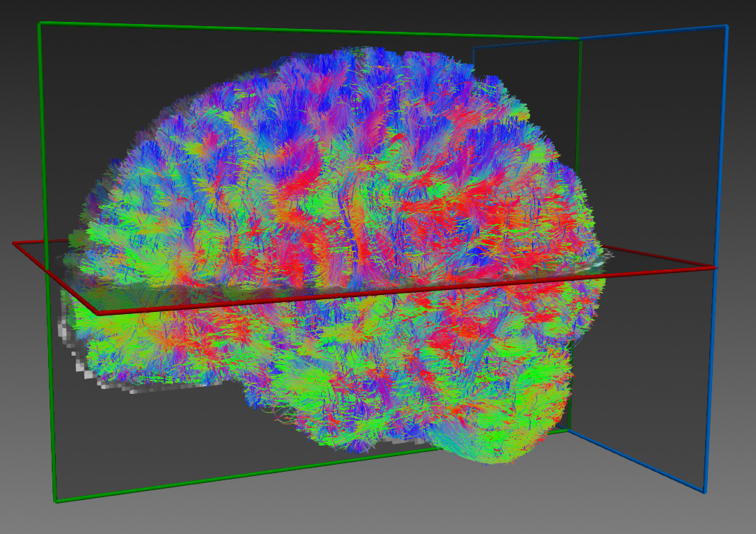
The dataset used throughout this showcase is an unfiltered whole-brain ensemble tractogram containing nearly 6 million streamlines (5,979,231 streamlines and 201,525,054 vertices) generated with tools from DIPY [Garyfallidis et al., 2014] and Scilpy [Renauld et al., 2026]. It is formed by concatenating tracking outputs from four distinct reconstruction and tracking algorithms: Diffusion Tensor Imaging (DTI), Euler Delta Crossings (EuDX), Deterministic CSD (DET), and Probabilistic Particle Filtering CSD (PROB).
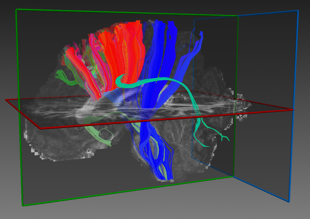
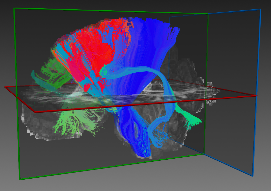
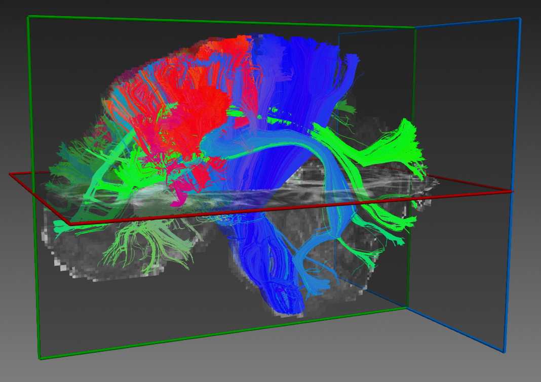
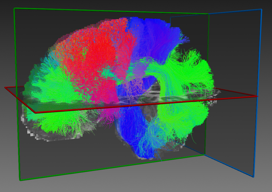
The showcase figures (the whole-brain ensemble and the tracking algorithm
bundles above) are rendered programmatically using FURY with axial and
mid-sagittal reference slices. The figure generation script is available on
GitHub as generate_showcase_figure.py.
Because tracking algorithm identifiers (algo) and Convex Optimization Modeling
for Microstructure Informed Tractography (COMMIT) signal weights (commit_weights)
[Daducci et al., 2015] are stored in independent Data Per Streamline (DPS)
arrays, this multi-gigabyte ensemble can easily be decomposed by algorithm,
filtered without decoding 3D geometry, and segmented into anatomical bundles
using sparse index sets stored in groups.
Note
Demonstration Dataset, Scripts & Context
Demonstration context: This ensemble tractogram serves as a technical benchmark for TRX file operations, memory-mapped I/O, and metadata manipulation. Tracking algorithms were run with default parameters without subject-specific fine-tuning, and bundle segmentations were performed using BundleSeg [St-Onge et al., 2023] without an atlas adapted to each individual tracking algorithm. Any visual imperfections or anatomical artifacts in the raw streamlines are methodological artifacts of this unrefined demonstration pipeline and are not relevant to the TRX file format itself.
Prerequisites: All code examples require
trx-pythonanddipy:pip install trx-python dipyDownload Dataset: The whole-brain demonstration file (
complete_tractogram.trx) can be downloaded directly from Google Drive.Download Python Scripts (also available in the repository on GitHub):
generate_showcase_figure.py: FURY figure rendering script with programmatic camera and dual anatomical slices.showcase_filtering.py: Metadata-driven filtering and group extraction.showcase_concatenation.py: Tractogram concatenation and assembly strategies.showcase_resizing.py: Pre-allocated memory map buffer management and resizing.
Metadata-driven filtering and group extraction#
Download showcase_filtering.py
A common challenge in large-scale tractography is filtering millions of streamlines according to quantitative criteria (such as microstructure signal weights from COMMIT or tracking algorithm identifiers) and extracting anatomical bundles.
In legacy formats (such as TRK or TCK), filtering requires decoding all streamline geometry into memory and looping sequentially over coordinate arrays. In TRX, metadata is organized across independent binary arrays:
Data per streamline (DPS): 1D or 2D typed arrays with one row per streamline (e.g.,
commit_weights.float32,algo.uint8).Data per vertex (DPV): Arrays with one value per streamline vertex (e.g., local FA, fiber orientation RGB colors).
Groups: Named index sets mapping streamlines to anatomical bundles (e.g.,
AF_L,CST_R,CC).Data per group (DPG): Metadata attributes attached to specific groups (e.g., bundle volume, mean FA).
Because these arrays are stored independently in the ZIP container, filtering queries can be evaluated directly on 1D NumPy arrays without touching the multi-gigabyte geometry array.
This layout would also simplify quality control (QC) and outlier filtering. Users could store streamline quality scores or pass/fail flags in DPS (e.g., COMMIT [Daducci et al., 2015] weights or TractOracle [Levesque et al., 2025] scores), point-wise metrics in DPV, valid and rejected streamlines in separate groups, and bundle-level QC summaries in DPG.
1. Loading and inspecting tractogram metadata#
We begin by loading the whole-brain tractogram. Memory mapping ensures that opening a multi-gigabyte TRX file is nearly instantaneous, as coordinate arrays are paged from disk on demand.
import logging
import os
from time import time
import numpy as np

from trx.trx_file_memmap import TrxFile, load, save
from dipy.io.streamline import save_tractogram

logging.basicConfig(
    level=logging.INFO,
    format="%(asctime)s [%(levelname)s] %(message)s",
    datefmt="%H:%M:%S",
)

logging.info("Loading whole-brain tractogram with metadata...")
trx = load("complete_tractogram.trx")
logging.info(
    "Loaded tractogram: %d streamlines, %d vertices",
    len(trx.streamlines),
    len(trx.streamlines._data),
)
2. Vectorized filtering on microstructure and algorithm labels#
We query two DPS arrays simultaneously:
commit_weights > 0: identifies streamlines that contribute non-zero signal in a microstructure optimization model.algo == 4: selects streamlines generated by probabilistic tractography (where algorithm codes are 1: DTI, 2: EuDX, 3: Deterministic, 4: Probabilistic).
Because trx.data_per_streamline exposes standard NumPy arrays, the intersection
is computed via vectorized boolean operations in milliseconds:
logging.info("Filtering streamlines by microstructure weight and tracking algorithm...")
timer = time()
ind_commit = np.argwhere(trx.data_per_streamline["commit_weights"] > 0).T[0]
ind_prob = np.argwhere(trx.data_per_streamline["algo"] == 4).T[0]
indices = np.intersect1d(ind_prob, ind_commit)
filtering_time = time() - timer

logging.info(
    "Identified %d / %d valid streamlines in %.3fs",
    len(indices),
    len(trx.streamlines),
    filtering_time,
)

# Subsetting via .select() preserves group definitions and group metadata (DPG)
timer = time()
sub_trx = trx.select(indices)
logging.info("Created sub-tractogram via .select() in %.3fs", time() - timer)

# Save filtered sub-tractogram directly as a standalone TRX file
save(sub_trx, "filtered_prob_commit.trx")
logging.info("Saved filtered sub-tractogram to 'filtered_prob_commit.trx'")
Important
Always use .select() when subsetting tractograms whose anatomical bundle
assignments must be preserved. Slicing with [] returns a view over geometry
only, discarding group definitions and DPG attributes.
3. Extracting and exporting anatomical bundle groups#
The filtered sub-tractogram retains the bundle hierarchy of the parent file.
We can iterate over bundle keys (such as AF_L, CST_R, CC), extract each
bundle with .get_group(), and export it to TRK or TRX:
groups_dir = "groups"
if not os.path.isdir(groups_dir):
    os.mkdir(groups_dir)

logging.info("Extracting and saving individual bundle groups...")
for key in sub_trx.groups.keys():
    group_trx = sub_trx.get_group(key)
    logging.info("  Bundle '%s': %d streamlines", key, len(group_trx.streamlines))
    sft = group_trx.to_sft()
    save_tractogram(sft, os.path.join(groups_dir, f"{key}.trk"))
    save(group_trx, os.path.join(groups_dir, f"{key}.trx"))

logging.info("Group extraction and export complete.")
Click to view expected output
09:19:02 [INFO] Loading whole-brain tractogram with metadata...
09:19:02 [INFO] Loaded tractogram: 5979231 streamlines, 201525054 vertices
09:19:02 [INFO] Filtering streamlines by microstructure weight and tracking algorithm...
09:19:02 [INFO] Identified 910604 / 5979231 valid streamlines in 0.136s
09:19:02 [INFO] Created sub-tractogram via .select() in 0.161s
09:19:10 [INFO] Saved filtered sub-tractogram to 'filtered_prob_commit.trx'
09:19:10 [INFO] Extracting and saving individual bundle groups...
09:19:10 [INFO]   Bundle 'AF_L': 1724 streamlines
09:19:11 [INFO]   Bundle 'SLF_L': 1687 streamlines
09:19:12 [INFO]   Bundle 'AF_R': 2840 streamlines
09:19:12 [INFO]   Bundle 'CST_L': 5058 streamlines
09:19:13 [INFO]   Bundle 'CC': 14736 streamlines
09:19:14 [INFO]   Bundle 'SLF_R': 1941 streamlines
09:19:14 [INFO]   Bundle 'CST_R': 3299 streamlines
09:19:15 [INFO] Group extraction and export complete.
Assembling tractograms from multiple sources#
Download showcase_concatenation.py
Studies that process cohorts, multi-seed tractography, or ensemble tracking frequently merge multiple streamline files into unified tractograms. TRX provides three assembly strategies with distinct performance profiles.
Setup and reference chunk#
We load a bundle tractogram (groups/CC.trx containing 14,736 streamlines and
877,275 vertices) to serve as a repeatable chunk for 100 iterations of merging:
import logging
from time import time
import numpy as np

from trx.trx_file_memmap import TrxFile, load, concatenate

logging.basicConfig(
    level=logging.INFO,
    format="%(asctime)s [%(levelname)s] %(message)s",
    datefmt="%H:%M:%S",
)

filename = "groups/CC.trx"
iteration = 100

logging.info("Loading reference tractogram '%s'...", filename)
trx = load(filename)
chunk_len = len(trx.streamlines)
chunk_pts = len(trx.streamlines._data)
logging.info("Reference chunk: %d streamlines, %d vertices", chunk_len, chunk_pts)
Strategy 1: Batch concatenation (concatenate)#
When all input objects are available in memory up-front, concatenate computes
the total streamline and vertex count across all inputs, creates a single
destination memory map, and copies data linearly in one pass.
logging.info("--- Strategy 1: Batch concatenation (known input list) ---")
timer = time()
concat_trx = concatenate([trx for _ in range(iteration)])
concat_time = time() - timer
logging.info(
    "Concatenated %dx chunks (%d streamlines) in %.3fs (%.1f streamlines/s)",
    iteration,
    len(concat_trx.streamlines),
    concat_time,
    len(concat_trx.streamlines) / concat_time,
)
Strategy 2: Incremental append (naive approach)#
When tractograms arrive sequentially (e.g. from an iterative tracking loop or
streamed computation), a naive approach is calling append_trx.append(trx) on
each step.
Because the destination file capacity is not known in advance, each call to
.append() must grow the underlying on-disk binary files and remap virtual
memory. Over many iterations, this creates heavy I/O overhead:
logging.info("--- Strategy 2: Naive incremental append (dynamic reallocation) ---")
append_trx = load(filename)
timer = time()
append_durations = []
for i in range(iteration - 1):
    step_timer = time()
    append_trx.append(trx)
    append_durations.append(time() - step_timer)

total_naive_time = time() - timer
logging.info(
    "Naive append %dx chunks: total %.3fs (avg per call: %.4fs)",
    iteration,
    total_naive_time,
    np.mean(append_durations),
)
Strategy 3: Pre-allocated memory map append (recommended)#
To achieve maximum throughput during streaming or iterative appending, TrxFile
can be initialized with an upper bound on streamline and vertex capacity.
Understanding allocated capacity vs. real data count#
Allocated capacity (
header["NB_STREAMLINES"],header["NB_VERTICES"]): The size of the underlying memory-mapped files on disk. Because the operating system only commits physical disk pages as bytes are written, pre-allocating large buffers incurs ~0 MB RAM overhead.Real data count (
_get_real_len()): The count of populated, valid streamlines and vertices.
Subsequent .append() calls write directly into the pre-allocated offsets and
positions arrays in place without resizing files. A single .resize() call at
the end trims the trailing unused pages back to the exact data length:
logging.info("--- Strategy 3: Pre-allocated memory map append (recommended) ---")
max_streamlines = 10_000_000
max_vertices = 500_000_000

# 1. Pre-allocate buffer capacity on disk (RAM overhead is ~0 MB via mmap)
timer = time()
alloc_trx = TrxFile(
    nb_streamlines=max_streamlines,
    nb_vertices=max_vertices,
    init_as=trx,
)
alloc_init_time = time() - timer
logging.info(
    "Pre-allocated buffer capacity: %d streamlines, %d vertices (init: %.4fs, RAM: ~0 MB)",
    max_streamlines,
    max_vertices,
    alloc_init_time,
)

# 2. Append chunks directly into pre-allocated memory-mapped arrays
timer = time()
prealloc_durations = []
for i in range(iteration):
    step_timer = time()
    alloc_trx.append(trx)
    prealloc_durations.append(time() - step_timer)

total_prealloc_time = time() - timer
real_strs, real_pts = alloc_trx._get_real_len()

logging.info(
    "Pre-allocated append %dx chunks: total %.3fs (avg per call: %.4fs)",
    iteration,
    total_prealloc_time,
    np.mean(prealloc_durations),
)
logging.info(
    "Buffer state before resize: allocated capacity = %d, real data count = %d",
    max_streamlines,
    real_strs,
)

# 3. Truncate trailing unused storage back to exact written content
timer = time()
alloc_trx.resize()
resize_time = time() - timer
logging.info(
    "Trimmed buffer to exact content (%d streamlines, %d vertices) in %.4fs",
    len(alloc_trx.streamlines),
    len(alloc_trx.streamlines._data),
    resize_time,
)
Click to view expected output
09:19:17 [INFO] Loading reference tractogram 'groups/CC.trx'...
09:19:17 [INFO] Reference chunk: 14736 streamlines, 877275 vertices
09:19:17 [INFO] --- Strategy 1: Batch concatenation (known input list) ---
09:19:18 [INFO] Concatenated 100x chunks (1473600 streamlines) in 0.812s (1814778.3 streamlines/s)
09:19:18 [INFO] --- Strategy 2: Naive incremental append (dynamic reallocation) ---
09:19:32 [INFO] Naive append 100x chunks: total 12.807s (avg per call: 0.1294s)
09:19:32 [INFO] --- Strategy 3: Pre-allocated memory map append (recommended) ---
09:19:32 [INFO] Pre-allocated buffer capacity: 10000000 streamlines, 500000000 vertices (init: 0.0006s, RAM: ~0 MB)
09:19:32 [INFO] Pre-allocated append 100x chunks: total 0.268s (avg per call: 0.0027s)
09:19:32 [INFO] Buffer state before resize: allocated capacity = 10000000, real data count = 1473600
09:19:33 [INFO] Trimmed buffer to exact content (1473600 streamlines, 87727500 vertices) in 0.3961s
Managing pre-allocated memory maps and resizing#
In streaming tracking algorithms and iterative pipelines, tractogram objects can exist in a partially filled state where buffer capacity exceeds valid data count. TRX supports adjusting capacity and data boundaries dynamically without re-reading coordinate data.
1. Downsizing streamline count#
When extracting a representative subset for visualization or testing,
resize(nb_streamlines=N) truncates the valid data count and buffer to N
streamlines. All associated DPV, DPS, and group entries are kept synchronized
automatically.
import logging
from trx.trx_file_memmap import load, save

logging.basicConfig(
    level=logging.INFO,
    format="%(asctime)s [%(levelname)s] %(message)s",
    datefmt="%H:%M:%S",
)

logging.info("Loading reference tractogram 'complete_tractogram.trx'...")
trx = load("complete_tractogram.trx")

# Create an independent, writable deepcopy of the memory maps
logging.info("Creating independent deepcopy of the tractogram...")
new_trx = trx.deepcopy()
logging.info(
    "Initial state: streamline_count = %d, vertex_count = %d",
    len(new_trx.streamlines),
    len(new_trx.streamlines._data),
)

# Downsize streamline count and buffer to 100,000
logging.info("Step 1: Downsizing to 100,000 streamlines...")
new_trx.resize(nb_streamlines=100_000)
logging.info(
    "After downsizing: streamline_count = %d, vertex_count = %d",
    len(new_trx.streamlines),
    len(new_trx.streamlines._data),
)
2. Expanding buffer capacity for incoming data#
If downstream processing will append additional streamlines, calling
resize(nb_streamlines=M) with M > N expands the underlying disk capacity.
The count of valid streamlines remains N = 100,000, ensuring no existing
streamlines are modified or invalidated:
# Expand buffer capacity to 1,000,000 without altering existing valid data
logging.info("Step 2: Expanding buffer capacity to 1,000,000 streamlines...")
new_trx.resize(nb_streamlines=1_000_000)
real_strs, real_pts = new_trx._get_real_len()
logging.info(
    "After capacity expansion: allocated buffer capacity = %d, valid data count = %d",
    new_trx.header["NB_STREAMLINES"],
    real_strs,
)
3. Final trimming and persistence#
Calling resize() without arguments performs automatic compaction: it scans the
offsets array, determines the exact boundary of valid streamlines (100,000),
and truncates the on-disk file to release unused capacity before saving:
# Truncate unused trailing capacity back to exact valid data length
logging.info("Step 3: Trimming buffer to exact data content...")
new_trx.resize()
logging.info(
    "After final trim: streamline_count = %d, vertex_count = %d",
    len(new_trx.streamlines),
    len(new_trx.streamlines._data),
)

# Persist trimmed tractogram and convert to StatefulTractogram
save_path = "resized_tractogram.trx"
save(new_trx, save_path)
logging.info("Persisted resized tractogram to '%s'", save_path)

sft = new_trx.to_sft()
logging.info(
    "Converted to StatefulTractogram: %d streamlines in %s space",
    len(sft),
    sft.space,
)
Click to view expected output
09:19:43 [INFO] Loading reference tractogram 'complete_tractogram.trx'...
09:19:44 [INFO] Creating independent deepcopy of the tractogram...
09:19:44 [INFO] Initial state: streamline_count = 5979231, vertex_count = 201525054
09:19:44 [INFO] Step 1: Downsizing to 100,000 streamlines...
09:19:44 [INFO] After downsizing: streamline_count = 100000, vertex_count = 4233395
09:19:44 [INFO] Step 2: Expanding buffer capacity to 1,000,000 streamlines...
09:19:44 [INFO] After capacity expansion: allocated buffer capacity = 1000000, valid data count = 100000
09:19:44 [INFO] Step 3: Trimming buffer to exact data content...
09:19:45 [INFO] After final trim: streamline_count = 100000, vertex_count = 4233395
09:19:45 [INFO] Persisted resized tractogram to 'resized_tractogram.trx'
09:19:45 [INFO] Converted to StatefulTractogram: 100000 streamlines in Space.RASMM space
Interoperability with legacy formats#
TRX files store streamline vertices in RAS+ world coordinates and embed
complete spatial geometry (VOXEL_TO_RASMM affine, voxel dimensions, and voxel
order) in header.json.
The matrix below summarizes the architectural and metadata capabilities of TRX compared to traditional tractography formats:
Capability / Feature |
TRX ( |
TrackVis ( |
MRtrix ( |
|---|---|---|---|
Spatial Coordinate System |
RAS+ World (mm) |
Voxel Corner (mm) |
RAS+ World (mm) |
Memory-Mapped Arrays ( |
Yes (random access, zero-copy) |
No (sequential generator only) |
No (sequential generator only) |
Data Per Streamline (DPS) |
Yes (arbitrary dtypes/dims) |
Yes (scalars only) |
No |
Data Per Vertex (DPV) |
Yes (arbitrary dtypes/dims) |
Yes (scalars only) |
No |
Overlapping Groups (Bundles) |
Yes ( |
No |
No |
Data Per Group (DPG) |
Yes ( |
No |
No |
Self-Contained Spatial Header |
Yes ( |
Yes (Header struct) |
No (Requires reference) |
Converting between TRX and DIPY’s StatefulTractogram is lossless for geometry:
import logging
from trx.trx_file_memmap import load
from dipy.io.streamline import save_tractogram

logging.basicConfig(
    level=logging.INFO,
    format="%(asctime)s [%(levelname)s] %(message)s",
    datefmt="%H:%M:%S",
)

logging.info("Loading TRX tractogram...")
trx = load("filtered_prob_commit.trx")

# Convert TRX to DIPY StatefulTractogram
sft = trx.to_sft()
logging.info(
    "Converted to StatefulTractogram: %d streamlines (Space: %s, Origin: %s)",
    len(sft),
    sft.space,
    sft.origin,
)

# Export geometry to legacy formats
save_tractogram(sft, "output_tractogram.trk")
save_tractogram(sft, "output_tractogram.tck")
logging.info("Exported tractogram to .trk and .tck")
Warning
While TRK supports per-streamline (DPS) and per-vertex (DPV) scalars, it cannot
represent overlapping bundle groups or per-group attributes (DPG). Formats like
TCK do not support metadata at all. Exporting to legacy formats will therefore
discard group hierarchy and bundle associations. Maintaining the master dataset
in .trx format preserves the complete metadata structure.